I’ve been working on a project lately that involved segmenting 2D attribute maps. The catch? I only had labels for a handful of pixels and needed a way to measure how confident the classification actually was. After a bit of digging, I stumbled upon Gaussian Mixture Models (GMMs)—they seemed like a perfect, elegant way to get those probabilistic results.

I couldn’t find an off-the-shelf version in scikit-learn that handled this specific semi-supervised setup (maybe it’s hiding in there somewhere!), but I actually saw that as a win. I really wanted to get under the hood of the math, and there’s no better way to learn than by building it yourself. So, here’s my attempt at breaking down the EM Algorithm as intuitively as possible, along with the resources that helped me along the way.

The problem

Say we are dealing with some data and each data point is associated with a random variable that we don’t observe. We call them Latent variables. For example (See Table 1), imagine I collected the data for heights of individuals in my locality but didn’t manage to record the gender or age of the individual. And for the sake of simplicity, let’s assume I know that my data clusters into three categories: men, women and children (class labels $\in [Man, Woman, Child]$). The goal is to get a probablistic classification for each data point: What is the probability that this data point belongs to the men category?

Idx	Height	Class
0	$x_1$	? ($z_1$)
1	$x_2$	? ($z_2$)
…	…	…
N-1	$x_{N-1}$	? ($z_{N-1}$)

So the task at hand is to estimate $P(z \mid x_i)$.

Parametric distributions and maximum likelihood estimates

Let’s assume that the full data, $x, z$ is distributed according to the probability distribution $P(x, z ; \theta)$, that is the distribution is defined with parameters $\theta$ (eg. mean and variance). In Bayesian terms, $P(x, z ; \theta)$ is the joint probability of observing the full data given the parameters $\theta$. Since we don’t observe the latent variables, we aim to maximize $P(x ; \theta)$ i.e. Evidence w.r.t latent variables.

Assuming independent and identially sampled data points, the Evidence is given by:

\[\text{Evidence} = \Pi_{i=0}^{N-1} P(x_i ; \theta)\]

Handling sums is much easier than handling products. Since logarithm is a monotonically increasing function, maximizing the evidence is same as maximizing logarithm of the evidence.

\[\begin{aligned} log(\text{Evidence}) &= log(\Pi_{i=0}^{N-1} P(x_i ; \theta)) \\ &= \sum_{i=0}^{N-1}log(P(x_i ; \theta)) \end{aligned}\]

Writing the evidence in terms of joint probability distribution:

\[\sum_{i=0}^{N-1}log(P(x_i ; \theta)) = \sum_{i=0}^{N-1}log(\int P(x_i, z ; \theta) dz)\]

Estimating the parameters thus is an optimization problem:

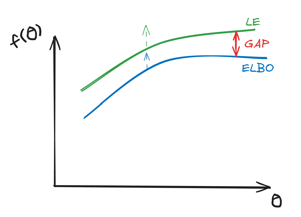
\[\begin{aligned} \theta &= \operatorname*{argmax}_{\theta} \text{(Evidence)} \\ &= \operatorname*{argmax}_{\theta} \sum_{i=0}^{N-1}log(\int P(x_i, z ; \theta) dz) \end{aligned}\]

Solving this optimization problem requires computing gradient of the objective, the Log Evidence (LE) with respect to the parameters and setting the gradient to zero. (first order optimality condition)

Let’s see what this entails:

\[\begin{aligned} \nabla_\theta \text{LE} &= \nabla_\theta(\sum_{i=0}^{N-1}log(\int P(x_i, z ; \theta) dz)) \\ &= \sum_{i=0}^{N-1} \nabla_\theta log(\int P(x_i, z ; \theta) dz) \\ &= \sum_{i=0}^{N-1} \frac{\nabla_\theta \int P(x_i, z ; \theta) dz}{\int P(x_i, z ; \theta)dz} \\ &= \sum_{i=0}^{N-1} \frac{\int \nabla_\theta P(x_i, z ; \theta) dz}{\int P(x_i, z ; \theta)dz} \end{aligned}\]

$\nabla_\theta \text{LE}$ is a vector as $\theta = [\theta_0, \theta_1, … \theta_K]$. In many probability models, $P$ usually take exponential forms. In the above setting, the form fo the gradient is very cumbersome. Setting the gradient to 0 leaves us with K equations where each equation has all of the integrals and the resulting system is highly coupled, most definitely non-linear.

Surrogate Objective - Evidence Lower Bounds (ELBO)

The problem above is that we end up with log of integrals. In order to simplify the optimization problem, we find a surrogate objective maximizing which results in the same parameters as the original objective.

A little mathematical manipulation coming up.

So we have the following objective:

\[\sum_{i=0}^{N-1}log(\int P(x_i, z ; \theta) dz)\]

Consider the integral: $\int P(x_i, z ; \theta) dz$. If we take an arbitrary probability distribution over $z$, we can re-write this as:

\[\begin{aligned} \int P(x_i, z ; \theta)dz &= \int \frac{P(x_i, z ; \theta)}{q(z)}q(z)dz \\ &= \mathbb{E}_{z\sim q(z)}[\frac{P(x_i, z ; \theta)}{q(z)}] \end{aligned}\]

So we can write LE as:

\[\text{LE} = \sum_{i=0}^{N-1}log(\mathbb{E}_{z\sim q(z)}[\frac{P(x_i, z ; \theta)}{q(z)}])\]

From here, we can use Jensen’s inequality and considering the fact that logarithm is a concave function, we have:

\[log(\mathbb{E}[X]) \geq \mathbb{E}[log(X)]\]

that leads to the inequality:

\[\text{LE} \geq \sum_{i=0}^{N-1}\mathbb{E}_{z \sim q(z)}[log(\frac{P(x_i, z ; \theta)}{q(z)})]\]

Given this Evidence Lower Bound (ELBO), maximing it with respect to $\theta$ also maximizes LE.

Let’s see if the gradient of ELBO is any easier:

\[\begin{aligned} \nabla_\theta \text{ELBO} &= \nabla_\theta \sum_{i=0}^{N-1}\mathbb{E}_{z \sim q(z)}[log(\frac{P(x_i, z ; \theta)}{q(z)})] \\ &= \nabla_\theta \sum_{i=0}^{N-1}\int log(\frac{P(x_i, z; \theta)}{q(z)})q(z)dz \\ &= \sum_{i=0}^{N-1}\int \nabla_\theta [log(\frac{P(x_i, z; \theta)}{q(z)})q(z)]dz \\ &= \sum_{i=0}^{N-1}\int \nabla_\theta log(P(x_i, z; \theta))q(z)dz \text{ -> as q(z) is independent of } \theta \end{aligned}\]

And as noted above, $P$ is usually modeled with exponentials (eg. Gaussian) in which case $log(P)$ simplifies, and the system of equations become relatively easy to solve.

Now let’s re-write the ELBO to reveal an interesting insight.

\[\begin{aligned} \text{ELBO} &= \sum_{i=0}^{N-1}\mathbb{E}_{z \sim q(z)}[log(\frac{P(x_i, z ; \theta)}{q(z)})] \\ &= \sum_{i=0}^{N-1}\mathbb{E}_{z \sim q(z)}[log(\frac{P(z\mid x_i; \theta)P(x_i; \theta)}{q(z)})] \\ &= \sum_{i=0}^{N-1}\mathbb{E}_{z \sim q(z)}[log(\frac{P(z\mid x_i; \theta)}{q(z)}) + log(P(x_i; \theta))] \\ &= \sum_{i=0}^{N-1}\mathbb{E}_{z \sim q(z)}[log(\frac{P(z\mid x_i; \theta)}{q(z)})] + \mathbb{E}_{z\sim q(z)}[log(P(x_i; \theta))] \text{ -> independent of } z\\ &= \sum_{i=0}^{N-1}\mathbb{E}_{z \sim q(z)}[log(\frac{P(z\mid x_i; \theta)}{q(z)})] + \sum_{i=0}^{N-1}log(P(x_i; \theta))\\ &= \sum_{i=0}^{N-1}\mathbb{E}_{z \sim q(z)}[log(\frac{P(z\mid x_i; \theta)}{q(z)})] + log(\text{Evidence}) \end{aligned}\]

Awesome!

We have:

\[\text{ELBO} = \sum_{i=0}^{N-1}\mathbb{E}_{z \sim q(z)}[log(\frac{P(z\mid x_i; \theta)}{q(z)})] + \text{LE}\]

and

\[\begin{aligned} \text{LE} &\geq \text{ELBO} \\ \implies \text{LE} &= \text{ELBO} + \text{GAP} \\ \implies \text{GAP} &= -\sum_{i=0}^{N-1}\mathbb{E}_{z \sim q(z)}[log(\frac{P(z\mid x_i; \theta)}{q(z)})] \\ &= \sum_{i=0}^{N-1}\mathbb{E}_{z \sim q(z)}[log(\frac{q(z)}{P(z\mid x_i; \theta)})] \end{aligned}\]

The GAP

If we analyse the GAP term:

\[\text{GAP} = \sum_{i=0}^{N-1}\mathbb{E}_{z \sim q(z)}[log(\frac{q(z)}{P(z\mid x_i; \theta)})]\]

and use Jensen’s inequality, we get:

\[\begin{aligned} \text{GAP} &\leq \sum_{i=0}^{N-1}log(\mathbb{E}_{z \sim q(z)}[\frac{q(z)}{P(z \mid x_i; \theta)}]) \\ &\geq \sum_{i=0}^{N-1}log(\mathbb{E}_{z \sim q(z)}[\frac{P(z \mid x_i; \theta)}{q(z)}] \\ \text{GAP} & \geq \sum_{i=0}^{N-1}log(\int \frac{P(z \mid x_i; \theta)}{q(z)} q(z) dz) = 0\\ \end{aligned}\]

as $\int P(z \mid x_i; \theta) dz = 1$ and $log(1) = 0$

P.S. The GAP is also called KL divergence.

The GAP = 0 when $q(z) = P(z \mid x_i; \theta)$, i.e. when $q(z)$ is equal to the posterior distribution.

Coordinate Ascent

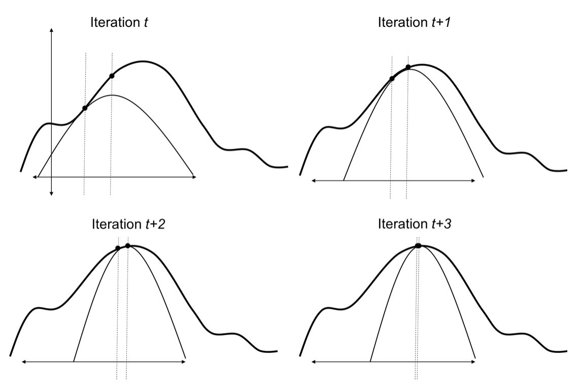
Without going into much details, its intuitive to see that to maximize the Evidence w.r.t $\theta$, we can first assume $\theta$ is constant and minimize the GAP, that is choose $q(z)$ to be posterior with fixed $\theta$ and then fix $q(z)$ to maximize the ELBO w.r.t $\theta$.

Here is an image from a nice reference 1, to demonstrate this, where the simpler curve is ELBO and the curve on top is the Evidence:

Wrapping up

In order for us to be able to compute things tractably, we need the posterior to be analytic. For GMM classification problem, we can get the posterior using a categorical prior and gaussian likelihood i.e. $z$ follows categorical distribution and given $z$, $x$ follows a normal distribution parametrised with some mean and covariance. EM algorithm is a good cadidate to solve such problems. For semi-supervised settings, the user provided labels set the categorical distribution for those particular data points and EM algorithm optimises for the remainder of parameters in the model.