Principal Component Analysis: Getting into Representation Learning

Real data is low dimensional

It is amazing how this simple statement can develop into a rich field that can be used to tackle a variety of problems. I came across the concept of representational learning through a very winding road. I should say from the existential crisis of watching LLMs get so good at knowledge work and questioning the value I bring at my work as a Computational Scientist. I don’t know why but one day I asked myself: “If AI takes my job of researching and implementing mathematical solutions to engineering problems, maybe my aim should be to equip myself with the tools to understand how AI does what it does!”. And then I ended up reading stuff about AI Interpretability for a couple of days. The biggest takeaway - AI learns concepts from data by representing things in ways that we as humans might find abstract but ways which make the concepts computable. Things behind most of the modern deep learning research and applications are all doing the same thing. So I felt its high time I dive deep into the what and why of these models/algorithms. And that is when I found this book - Principles and Practice of Deep Represenation Learning. It had the right amount of mathematical rigour I love and the right content I imagine I would need to get good at the things I see myself doing in the future. I hope to document my learnings through this blog. Unlike my time in university, I am not bound by exams or deadlines. So I am going to take my sweet time diving deep and probably re-visiting the concepts I already know with the rigour and intuition that I wish I had time for :)

Low-Dimensional Subspace

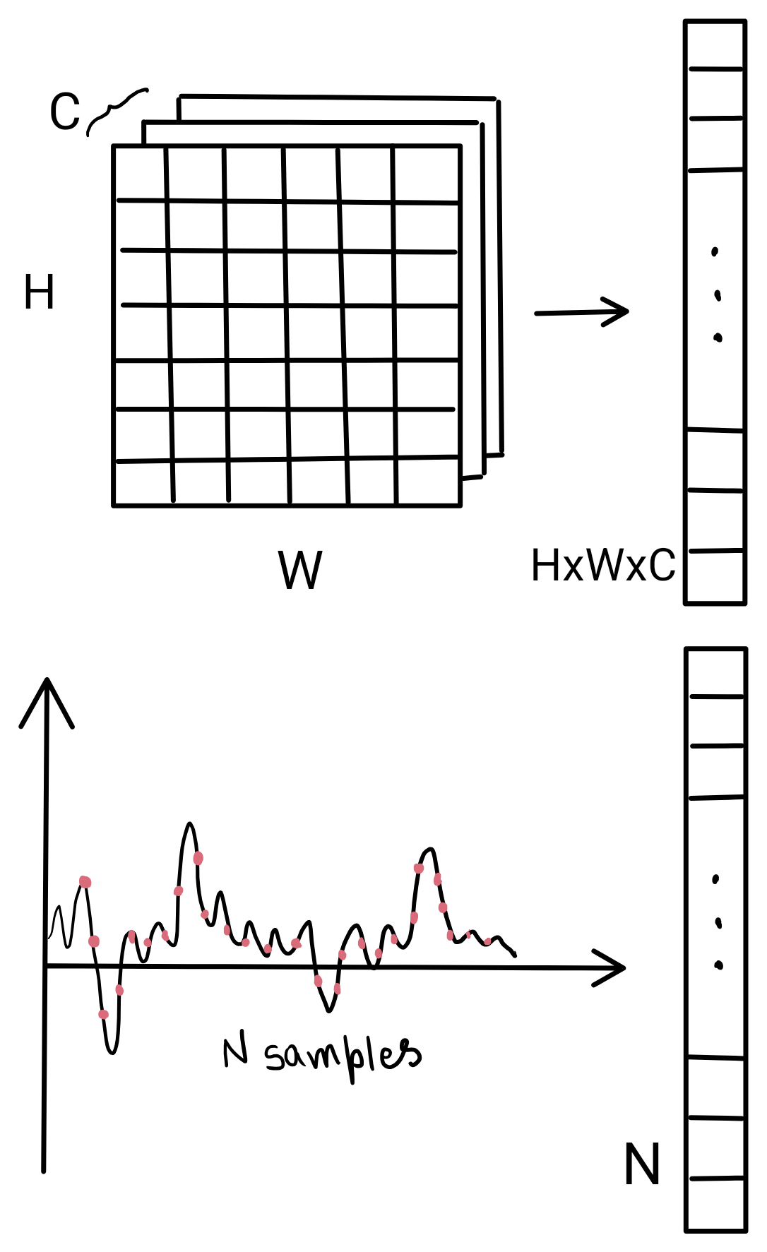
As in any most mathematical treatments, the book starts with a simplification of the the general statement “Real data is low dimensional”. Real data that we work with in the digital world is represented as a discrete signal. Be it images (color values on a pixel grid), audio (amplitude values at discrete time samples) etc. It’s easy to see how they can be represented at vectors in a high-dimensional space.

If we consider the dimension of the space that the data comes from as \(D\), low-dimensionality of the data means that these vectors don’t occupy the entirety of \(\mathbb{R}^D\). Instead we assume that the data is restricted to a particular region within \(\mathbb{R}^D\), a sub-manifold. In the first part of the book, we make a further simplifying assumption: the data comes from a linear subspace \(\mathbb{R}^d\) of dimension \(d \ll D\) within \(\mathbb{R}^D\). It’s easy to visualise if we consider \(D=3\).

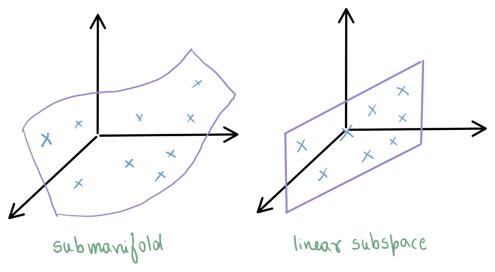
Note that the definition of subspace requires that the \(\bar{0}\) belongs to the dataset. In general, we could do something like subtracting the mean from the data and then model it with this assumption. With that assumption, the mathematical model describing the data would be:

\[\begin{equation} \bar{x}_i = U \bar{z}_i + \bar{\epsilon}_i \end{equation}\]

Where

\(\bar{x}_i \in \mathbb{R}^D\) is the data

\(U \in \mathbb{R}^{D \times d}\) is the matrix whose columns spans subspace

\(\bar{z}_i \in \mathbb{R}^d\) is the latent code

\(\bar{\epsilon}_i \in \mathbb{R}^D\) is noise

Given \(N\) such data points, the goal is to find the matrix \(U\) (the basis of the subspace) and the latent codes \(\bar{z}_i\) that closely approximate the observed data under the modeling assumption. This is equivalent to minimizing the difference between model predicted and the observed data or de-noising the data to fit the modelling assumption.

Solving the problem

In this section, I try to derive the steps involved in solving the above problem in line with the book but also expanding steps to derive in as much detail as I found necessary to get full intuition. I might go into a rabbit hole of working out concepts that form the foundations so that I can have everything in place. Will put those tangents in a foldable section for you to skip if not interested.

\[\begin{equation} \begin{aligned} & \underset{U, \{z_i\}}{\text{minimize}} \quad \frac{1}{N} \sum_{i=1}^{N} \|x_i - U z_i\|_2^2 \\ & \text{such that} \quad U^T U = I \end{aligned} \end{equation}\]

For given \(U\), the optimal \(\bar{z}_i\) can be found as follows:

Each term is +ve and independent. So we can minimize each term individually

Expanding the \(L_2\) norm.

\[\begin{aligned} \|\bar{x}_i - U \bar{z}_i\|_2^2 &= (\bar{x}_i - U \bar{z}_i)^T (\bar{x}_i - U \bar{z}_i) \\ &= (\bar{x}_i^T - \bar{z}_i^T U^T)(\bar{x}_i - U \bar{z}_i) \\ &= \bar{x}_i^T \bar{x}_i - 2 \bar{z}_i^T U^T \bar{x}_i + \bar{z}_i^T \underbrace{U^T U}_{I} \bar{z}_i \\ &= \bar{x}_i^T \bar{x}_i - 2 \bar{z}_i^T U^T \bar{x}_i + \bar{z}_i^T \bar{z}_i \end{aligned}\]

Taking derivative w.r.t \(\bar{z}_i\) and equating to \(0\)

With optimal \(\bar{z}_i = U^T \bar{x}_i\), we can now solve

\[\begin{equation} \underset{U}{\text{minimize}} \quad \frac{1}{N} \sum_{i=1}^{N} \|\bar{x}_i - U U^T \bar{x}_i\|_2^2 \end{equation}\]

Expanding the \(L_2\) norm again

\[\begin{aligned} \|\bar{x}_i - U U^T \bar{x}_i\|_2^2 &= (\bar{x}_i - U U^T \bar{x}_i)^T (\bar{x}_i - U U^T \bar{x}_i) \\ &= (\bar{x}_i^T - \bar{x}_i^T U U^T)(\bar{x}_i - U U^T \bar{x}_i) \\ &= \bar{x}_i^T \bar{x}_i - \bar{x}_i^T U U^T \bar{x}_i - \bar{x}_i^T U U^T \bar{x}_i \\ &\quad + \bar{x}_i^T U \underbrace{U^T U}_{I} U^T \bar{x}_i \\ &= \bar{x}_i^T \bar{x}_i - 2 \bar{x}_i^T U U^T \bar{x}_i + \bar{x}_i^T U U^T \bar{x}_i \\ &= \underbrace{\bar{x}_i^T \bar{x}_i}_{\text{Independent of } U} - \bar{x}_i^T U U^T \bar{x}_i \end{aligned}\]

or

such that \(U^T U = I\)

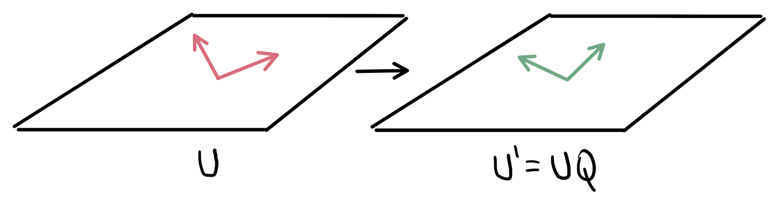
There is an important observation regarding the objective. Consider an orthonormal matrix \(Q \in \mathbb{R}^{d \times d}\). The matrix defined as \(U' = U Q\). Its easy to see that

i.e each column of \(U'\) is a linear combination of the columns of \(U\). Therefore \(col(U') \subseteq col(U)\). Since \(Q\) is orthonormal, it is invertible or full rank which means the linear combinations don’t collapse \(\Rightarrow col(U') = col(U)\). Added to that, \(U' {U'}^T = (UQ) (UQ)^T = U Q Q^T U^T\). Since \(Q^T Q = I\) and \(Q\) is square, \(Q^{-1} = Q^T\) and \(Q Q^T = I\) So \(U' {U'}^T = U Q Q^T U^T = U U^T\). Meaning the objective value is same and the problem doesn’t have a unique solution.

We reformulate the objective to make it convenient.

Let \(U^T \bar{x}_i = \bar{v}_i\)

The diagonal entry of \(i^{th}\) row \(= \sum_{j=1}^{N} v_{ji}^2\)

And \(\operatorname{trace} = \sum_{i=1}^{N} \sum_{j=1}^{N} v_{ji}^2 = \sum_{j=1}^{N} \|\bar{v}_j\|_2^2 = \sum_{j=1}^{N} \bar{v}_j^T \bar{v}_j\)

So the objective can be written as:

\[\begin{equation} \begin{aligned} &\operatorname*{maximize}_{U} \operatorname{trace}\left(U^T \frac{X X^T}{N} U\right) \\ &\text{such that } U^T U = I \end{aligned} \end{equation}\]

Properties of \(M = \frac{X X^T}{N}\)

• We notice that \(M\) is symmetric. \((X X^T)^T = (X^T)^T X^T = X X^T\), i.e. \(M^T = M\)
• Let \(\bar{v}\) be a complex vector. Let \(C = \bar{v}^* M \bar{v}\) where \(\bar{v}^*\) is the transpose of complex conjugate & \(\bar{v}^* \bar{v} = \|\bar{v}\|^2\). \(C^* = (\bar{v}^* M \bar{v})^* = \bar{v}^* M^* \bar{v}\). We notice \(M\) is symmetric. We also notice that \(M\) is real. \(\therefore M^* = M \implies C^* = \bar{v}^* M \bar{v} = C \implies C\) is real.
• If \(\bar{v}\) is an eigenvector, \(M \bar{v} = \lambda \bar{v}\) \(C = \bar{v}^* M \bar{v} = \bar{v}^* \lambda \bar{v} = \lambda \bar{v}^* \bar{v} = \lambda \|\bar{v}\|^2\). \(C\) is real, \(\|\bar{v}\|^2\) is real \(\implies \lambda\) is real. Real symmetric matrix has real eigen values.
• Let \(\bar{v} = \bar{a} + i\bar{b}\). Then \(M(\bar{a} + i\bar{b}) = \lambda(\bar{a} + i\bar{b})\) \((M - \lambda I)(\bar{a} + i\bar{b}) = 0\). \(\lambda\) being the eigenvalue, \(\det(M - \lambda I) = 0 \implies \bar{a} + i\bar{b}\) has non trivial solution, especially, \(\bar{a}\) has non trivial solution. So we can find real eigenvectors of \(M\) for every real eigenvalue.

• Consider another eigenvector \(\bar{u}\) such that \(M \bar{u} = \mu \bar{u}\). We have: \(\bar{v}^T M \bar{u} = \mu \bar{v}^T \bar{u} \implies (M^T \bar{v})^T \bar{u} = \mu \bar{v}^T \bar{u} \implies (M \bar{v})^T \bar{u} = \mu \bar{v}^T \bar{u}\) \(\implies \lambda \bar{v}^T \bar{u} = \mu \bar{v}^T \bar{u} \implies (\lambda - \mu) \bar{v}^T \bar{u} = 0\). \(\lambda \neq \mu \implies \bar{v}^T \bar{u} = 0\) Symmetric matrix has orthogonal eigenvectors.

• If we use the definition of \(M = \frac{x x^T}{N}\), we have
  $$\bar{v}^T M \bar{v} = \bar{v}^T \frac{x x^T}{N} \bar{v} = \frac{1}{N} (x^T \bar{v})^T (x^T \bar{v})$$
  $$= \frac{1}{N} \| x^T \bar{v} \|^2 \geqslant 0$$

  For eigenvector, \(M \bar{v} = \lambda \bar{v} \Rightarrow \bar{v}^T M \bar{v} = \bar{v}^T \lambda \bar{v} = \lambda \| \bar{v} \|^2\)

So \(M\) is Positive Semidefinite and all the eigenvalues are \(\geqslant 0\)

• What do 0 eigenvalues mean? We proved that real symmetric positive semidefinite matrix has real eigenvalues \(\geqslant 0\), and corresponding real orthogonal eigenvectors. \(M = \frac{x x^T}{N} \in \mathbb{R}^{D \times D}\). So the \(D\) eigenvectors span the whole of \(\mathbb{R}^D\). Any vector \(\bar{\alpha}\) in \(\mathbb{R}^D\) can be written as \(\sum_{i=1}^D \alpha_i \bar{v}_i\). If \(M\) has zero eigenvalues, \(M \bar{\alpha} = M \sum_{i=1}^D \alpha_i \bar{v}_i = \sum_{i=1}^D \alpha_i M \bar{v}_i\). The terms involving eigenvectors corresponding to \(0\) eigenvalues vanish as \(M \bar{v} = \lambda \bar{v} = 0\). So \(M\) collapses dimensions. How many zero eigenvalues therefore tell us the dimension of nullspace of \(M\). From rank-nullity theorem, if no. of zero eigenvalues = nullity = \(n\), \(n + \text{rank} = D \Rightarrow \text{rank}(M) = D - n\)

Optimization with Equality Constraint:

Lagrange Multiplier method

Optimize \(f(\bar{x})\), subject to \(g(\bar{x})=0\), \(x \in \mathbb{R}^D\). Consider a curve in \(\mathbb{R}^D\) parametrised as \(\bar{r}(t)\). We want those specific curves which satisfy \(g(\bar{r}(t)) = 0\). Taking derivative w.r.t. \(t\):

Now along \(r(t)\), \(\bar{x}^* = r(0)\) is the minimum.

So \(\dot{\bar{r}}(t)\) at \(t=0\) is \(\perp\) to both \(\nabla g\) & \(\nabla f\). \(\therefore\) at \(\bar{x}^*\): \(\nabla f = \lambda \nabla g\) or \(\nabla f - \lambda \nabla g = 0\)

We define Lagrangian as \(f - \lambda g\). At \(\bar{x}^*, \lambda^*\), \(\nabla \mathcal{L} = 0\) i.e

Finding a solution

Let \(U = [\bar{u}_1, \bar{u}_2 \dots \bar{u}_d]\). Then:

The constraints are \(\bar{u}_i^T \bar{u}_i = 1\) and \(\bar{u}_i^T \bar{u}_j = 0 \; j \neq i\). Setting up the Lagrangian:

Left multiplying (A) with \(\bar{u}_i^T\), we get:

The objective is to maximise \(\text{trace}(U^T M U) = \sum_{i=1}^d \bar{u}_i^T M \bar{u}_i\). Since \(\bar{u}_i\) are unit eigenvectors, \(\text{trace}(U^T M U) = \sum_{i=1}^d \bar{u}_i^T \lambda_i \bar{u}_i = \sum_{i=1}^d \lambda_i \bar{u}_i^T \bar{u}_i = \sum_{i=1}^d \lambda_i\).

Maximizing the objective therefore means picking the top \(d\) eigenvectors of \(M\) i.e. eigenvectors corresponding to largest \(d\) eigenvalues (all of which are \(\ge 0\)).

Geometrical interpretation:

We derived that one solution to the problem is \(U\) made up of top \(d\) eigenvectors of \(M = \frac{X X^T}{N}\) and the corresponding latent codes are \(\bar{z}_i = U^T \bar{x}_i\).

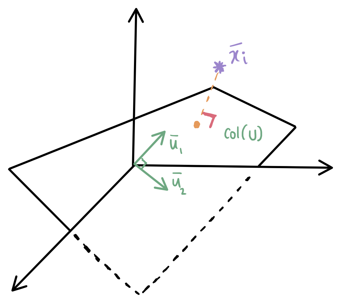
The denoised data point is therefore \(U U^T \bar{x}_i\). To see what it means geometrically, consider \(\bar{u}_i\). The denoised data point is \(\bar{u}_i (\bar{u}_i^T \bar{x}_i) = (\bar{u}_i^T \bar{x}_i) \bar{u}_i\), which is the projection of \(\bar{x}_i\) on \(\bar{u}_i\). \(U U^T \bar{x}_i\) therefore is the orthogonal projection of \(\bar{x}_i\) onto the subspace spanned by top \(d\) eigenvectors of \(M\).

How do we pick \(d\)?

Lets figure this out by taking an example that is easy to visualize. Let \(\bar{x}_i \in \mathbb{R}^3\). \(\therefore D=3\) and \(M = \frac{X X^T}{N} \in \mathbb{R}^{3 \times 3}\). \(M\) will have \(\lambda_i \ge 0\) and corresponding \(\bar{v}_i, i \in \{1, 2, 3\}\).

Lets take an extreme case where all \(\bar{x}_i\) lie on a line in 3D i.e \(\bar{x}_i = c_i \hat{a}\) (note we want \(\bar{x}_i\) to lie on a subspace so line passes through origin). Lets also assume we don’t know this and model it as coming from a 2D subspace. i.e we chose \(d=2\). Now,

\[\begin{aligned} M = X X^T / N &= \frac{1}{N} \begin{bmatrix} c_1 \hat{a} & c_2 \hat{a} & \dots & c_N \hat{a} \end{bmatrix} \begin{bmatrix} - c_1 \hat{a} - \\ - c_2 \hat{a} - \\ \vdots \\ - c_N \hat{a} - \end{bmatrix} \\ &= \left( \frac{\sum_{i=1}^N c_i^2}{N} \right) \hat{a} \hat{a}^T = \overline{c^2} \ \hat{a} \hat{a}^T \end{aligned}\]

If \(M = AB\), \(\text{col}(M) \subseteq \text{col}(A) \Rightarrow \text{rank}(M) \le \text{rank}(A)\) \(M^T = B^T A^T \Rightarrow \text{rank}(M^T) = \text{rank}(M) \le \text{rank}(B^T) = \text{rank}(B)\) \(\therefore \text{rank}(M) \le \min(\text{rank}(A), \text{rank}(B))\).

\(\hat{a}\) & \(\hat{a}^T\) are rank \(1\) matrices. \(\therefore M\) has rank \(1\). From previous discussion, \(\text{rank} + \text{nullity} = 3\) \(\text{nullity} = 3 - 1 = 2\)

Number of zero eigenvalues \(= 2\)

We can easily see that one of the eigenvectors is \(\hat{a}\) \(M \hat{a} = (\overline{c^2} \,\, \hat{a} \hat{a}^T) \hat{a} = \overline{c^2} \,\, \hat{a} \quad \text{as } \hat{a}^T \hat{a} = 1\) \(\therefore \hat{a}\) is eigenvector with eigen value \(\overline{c^2}\). The other eigenvalues are \(0\). So of the three eigenvectors that span \(\mathbb{R}^3\), one vector is \(\hat{a}\) and the two remaining span the plane \(\perp \hat{a}\). We could pick either of these as the second column of \(U\) for PCA. The latent codes would then be of the form \(\bar{z}_i = U^T \bar{x}_i = \begin{bmatrix} -\hat{a}- \\ -\bar{v}- \end{bmatrix} [\bar{x}_i] = \begin{bmatrix} c_i \\ 0 \end{bmatrix}\)

If \(\bar{x}_i\) were noisy and deviated slightly from the line, we would have a second non-zero eigenvalue, albeit small in magnitude.

So a way to pick reasonable \(d\) is to find the eigenvalues of \(M\), rank them based on magnitude and pick \(d\) after which the magnitude drastically drops.

Finding the Eigenvectors : Power Iteration

Consider an iterative scheme \(\bar{z}_t = \frac{M\bar{z}_{t-1}}{\|M\bar{z}_{t-1}\|}\)

Expanding telescopically, \(\bar{z}_t = \frac{M^t \bar{z}_0}{\prod_{i=0}^{t-1} \|M\bar{z}_i\|} = \frac{M^t \bar{z}_0}{\|M^t \bar{z}_0\|} \text{ as } \bar{z}_t \text{ is unit vector}\)

\(M\) has eigenvectors \(\bar{v}_i \in \mathbb{R}^D\) that span \(\mathbb{R}^D\). \(\therefore \bar{z}_0 = \sum_{i=1}^{D} \alpha_i \bar{v}_i\)

\[\begin{aligned} \bar{z}_t &= \frac{M^t \sum_{i=1}^{D} \alpha_i \bar{v}_i}{\|M^t \sum_{i=1}^{D} \alpha_i \bar{v}_i \|} = \frac{\sum_{i=1}^{D} \alpha_i M^t \bar{v}_i}{\| \sum_{i=1}^{D} \alpha_i M^t \bar{v}_i \|} = \frac{\sum_{i=1}^{D} \alpha_i \lambda_i^t \bar{v}_i}{\| \sum_{i=1}^{D} \alpha_i \lambda_i^t \bar{v}_i \|} \end{aligned}\]

If \(\lambda_1 \geqslant \lambda_2 \geqslant \lambda_3 \dots \geqslant \lambda_D\)

\[\bar{z}_t = \frac{\sum_{i=1}^{D} \alpha_i \lambda_i^t \bar{v}_i}{\sqrt{\underbrace{\sum_{i=1}^{D} \alpha_i^2 \lambda_i^{2t} \|\bar{v}_i\|^2}_{\text{as } \bar{v}_i^T \bar{v}_j = 0}}}\]

Factoring out \(\lambda_1^t\)

\[\bar{z}_t = \frac{\lambda_1^t (\alpha_1 \bar{v}_1 + \sum_{i=2}^{D} \alpha_i \left(\frac{\lambda_i}{\lambda_1}\right)^t \bar{v}_i)}{|\lambda_1^t| \sqrt{\alpha_1^2 \|\bar{v}_1\|^2 + \sum_{i=2}^{D} \alpha_i^2 \left(\frac{\lambda_i}{\lambda_1}\right)^{2t} \|\bar{v}_i\|^2}}\]

As \(\lambda_1 > 0\), \(|\lambda_1|^t = \lambda_1^t\). Also, \(\frac{\lambda_i}{\lambda_1} < 1; i \neq 1\) \(\therefore\) as \(t \to \infty\), \(\left(\frac{\lambda_i}{\lambda_1}\right)^t \to 0\)

As \(t \to \infty\), $$\bar{z}_t \to \frac{\alpha_1 \bar{v}_1}{

\alpha_1

|\bar{v}_1|} = \text{sgn}(\alpha_1) \hat{\bar{v}}_1$$

The iteration converges to the top eigenvector of \(M\) (along or opposite based on sign of \(\alpha\)). To find other eigenvectors, we effectively want \(M' \in \mathbb{R}^{D \times D}\) such that the eigenvalue corresponding to \(\bar{v}_1\) be zero but preserves every other eigenvalue of \(M\). \(\therefore M'\) should have nullity \(= 1\) and nullspace is spanned by \(\bar{v}_1\). \(M' \bar{v}_1 = 0\) and \(M' \bar{v}_i = \lambda_i \bar{v}_i; i \neq 1\).

Given arbitrary vector \(\bar{z}\), we want \(M'\) such that it is projected in subspace \(\perp\) to \(\bar{v}_1\), apply \(M\) and then squash it back to subspace.

Projector \(P\): \(I - \bar{v}_1 \bar{v}_1^T\) (remove component along \(\bar{v}_1\)). Apply \(M\) and project back.

\[\begin{aligned} \therefore M' &= P M P \\ &= (I - \bar{v}_1 \bar{v}_1^T) M (I - \bar{v}_1 \bar{v}_1^T) \\ &= (I - \bar{v}_1 \bar{v}_1^T)(M - M \bar{v}_1 \bar{v}_1^T) \\ &= (I - \bar{v}_1 \bar{v}_1^T)(M - \lambda_1 \bar{v}_1 \bar{v}_1^T) \\ &= M - \lambda_1 \bar{v}_1 \bar{v}_1^T - \bar{v}_1 \underbrace{\bar{v}_1^T M}_{(M \bar{v}_1)^T} + \lambda_1 \bar{v}_1 \underbrace{\bar{v}_1^T \bar{v}_1}_{1} \bar{v}_1^T \\ &= M - \lambda_1 \bar{v}_1 \bar{v}_1^T - \bar{v}_1 (M \bar{v}_1)^T + \lambda_1 \bar{v}_1 \bar{v}_1^T \\ &= M - \lambda_1 \bar{v}_1 \bar{v}_1^T - \bar{v}_1 \lambda_1 \bar{v}_1^T + \lambda_1 \bar{v}_1 \bar{v}_1^T \\ M' &= M - \lambda_1 \bar{v}_1 \bar{v}_1^T \end{aligned}\]

We can check what happens to the eigen vectors of \(M\) under \(M'\)

\[\begin{aligned} M' \bar{v}_1 &= M \bar{v}_1 - \lambda_1 \bar{v}_1 \bar{v}_1^T \bar{v}_1 = \lambda_1 \bar{v}_1 - \lambda_1 \bar{v}_1 = 0 \\ M' \bar{v}_i, i \neq 1 &= M \bar{v}_i - \lambda_1 \bar{v}_1 \bar{v}_1^T \bar{v}_i = M \bar{v}_i = \lambda_i \bar{v}_i \end{aligned}\]

Repeat this till we get the top \(d\) eigenvectors

Probabilistic PCA

We now consider data as samples of a random variable \(\bar{x}\) taking values in \(\mathbb{R}^D\). \(\bar{x}\) is said to have an approximate low rank statistical structure iff \(\exists U \in \mathbb{R}^{D \times d} : U^T U = I\), \(\bar{z}\) a random vector in \(\mathbb{R}^D\) and small random vector \(\bar{\epsilon} \in \mathbb{R}^D\) where \(\bar{z}\) & \(\bar{\epsilon}\) are independent, and

Goal is to recover \(U\). The objective here would be

Following same steps as we did for PCA, we end up with \(M = \mathbb{E} [\bar{x} \bar{x}^T]\) and columns of \(U\) as top \(d\) eigenvectors of \(M\).

\(\begin{aligned} \operatorname{Cov}(\bar{x}) &= \mathbb{E}[(\bar{x} - \bar{\mu})(\bar{x} - \bar{\mu})^T] = \mathbb{E}[(\bar{x} - \bar{\mu})(\bar{x}^T - \bar{\mu}^T)] \\ &\Rightarrow \mathbb{E}[\bar{x} \bar{x}^T - \bar{x} \bar{\mu}^T - \bar{\mu} \bar{x}^T + \bar{\mu} \bar{\mu}^T] \end{aligned}\) \(\mathbb{E}[\bar{x}] = \mathbb{E}[U \bar{z} + \bar{\epsilon}] = U \mathbb{E}[\bar{z}] + \mathbb{E}[\bar{\epsilon}]\). If \(\bar{z}\) & \(\bar{\epsilon}\) are zero mean, \(\mathbb{E}[\bar{x}] = \bar{\mu} = \bar{0}\)

Conclusion

I believe I now have enough intuition of the problem we are trying to solve and got to revise some core tools and concepts which will help in later sections. See you there!